Key Terms
- Agent: the object we are observing for finding the best optimal policies.
- States: $s_i$ The state space is $\mathcal{S} = {s_1, \cdots s_n}$
- Actions: $a_i$ The action space is $\mathcal{A} = {a_1,\cdots, a_m}$
- State Transition: $s_1 \xrightarrow{a_2} s_2$
- Rewards: the feedback from the environment. Positive reward will encourage an agent to take the corresponding action, and vice versa for negative reward. (Human-Machine Interface)
- Returns: the return of trajectory is the sum of rewards collected along the trajectory. (Also known as Total rewards or cumulative reward). Returns consists immediate reward and future reward.
- Discounted Returns: A discounted factor is applied for infinitely long trajectories. It can also adjust the emphasis on near- or far-future rewards.
- Policies: Policy (stochastic in general, but sometimes deterministic) tells the agent which actions to take at every state, which can be denoted as arrow.
- Trajectory: a state-action-reward chain. $s_1 \xrightarrow[r=0]{a_2} s_2 \xrightarrow[r=0]{a_3} s_5 \xrightarrow[r=0]{a_3} s_8 \xrightarrow[r=1]{a_2} s_9 .$ There is infinite-length(horizon) trajectory except for finite trajectory. So for finite returns and infinite reward.
- Immediate Rewards: reward obtained after taking an action at the initial state.
- Future Rewards: reward obtained after leaving the initial state.
- Episodes: a finite trajectory with terminal states whose result trajectory is an episode.
- episodic task/continuing task: whether terminal states exist. The episodic tasks can be mathematically converted to continuing tasks by defining the processes after reaching terminal states.
- visit: every time a state-action pair appears in an episode, it is called a visit of state-action pair.
- Behavior Policy: it is used to generate experience samples.
- Target Policy: it is constantly updated to converge to an optimal policy.
- On-policy: When the behavior policy is equal to the target policy.
- Off-policy: When the behavior policy is different from the target policy. off-policy learning can learn optimal policies based on the experience samples generated by other policies.
- Experience replay: The draw of samples is called experience replay, which should follow a uniform distribution. The main function of experience replay is to break the correlation of a sequence of action-state pairs. After we have collected some experience samples, we do not use these samples in the order they were collected. They are stored at the replay buffer. $(s, a, r, s’)$ is the experience sample and $\mathcal{B}= {(s, a, r, s’)}$ is the replay buffer. Every time updating the network we will draw a mini-batch from the replay buffer.
- Policy Evaluation: Policy Evalution is the process calculating state value or action value based on given policy when the system dynamics is given or samplable. Since the state value can be used to evaluate a policy, solving the state values from the Bellman Equation is policy evaluation. Basically, the task of Policy Evalution is to solve the Bellman Equation.
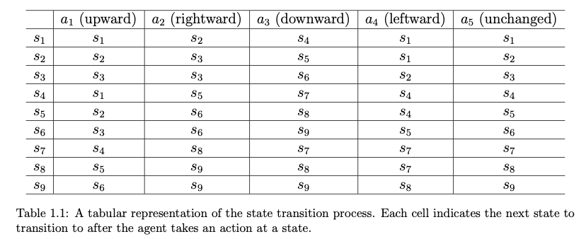
Two ways to express Deterministic State Transition:
- Table (only deterministic state transition)

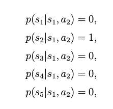
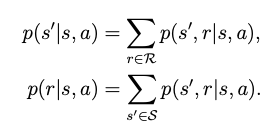
Probability Expression

Key Concept & Key Tool
Concepts
State Value
It’s the expected return (average reward / total reward) that an agent can obtain when starting from a state through following a given policy. It can be taken as a metric to evaluate the goodness of a policy.
The returns can be utilized to evaluate policies. However, it is inapplicable to stochastic systems, because starting from one state will lead to different returns.
Therefore, returns → state values
$$
S_t \xrightarrow{A_t} S_{t+1}, R_{t+1}
$$
$S_t, A_t, S_{t+1}, R_{t+1}$ are all random variables. $A_t \in \mathcal{A}(S_t)$ is the action taken by following Policy $\pi$. The immediate reward is $R_{t+1} \in \mathcal{R}(S_t,A_t)$. Therefore, the discounted return along the trajectory is
$$
G_t = R_{t+1} + \gamma R_{t+2} + \gamma^2 R_{t+3}+ \cdots,
$$
where the $G_t$ is a random variable, which can be obtained by calculating expected value. Since the policy is given, $A_t$ is not a random variable here.
$$
v_\pi(s) = \mathbb{E}[G_t|S_t = s]
$$
This expected value $v_\pi (s)$ is called the state-value function or state value of $s$ .
Motivating Example:

The return by following the first policy is $\text{return}_{1} = 0 + \gamma1 + \gamma 1 + \cdots = \frac{\gamma}{1 - \gamma}$;
The return by following the second policy is $\text{return}_2 = -1 + \frac{\gamma}{1- \gamma}$;
The thrid return is $\text{return}_3 = 0.5 \times \text{return}_1 + 0.5 \times \text{return}_2 = -0.5 + \frac{\gamma}{1- \gamma}$
The idea to calculate returns:
$$
v_1 = r_1 + \gamma (r_2 + \gamma r_3 + \cdots) = r_1 + \gamma v_2
$$
$$
v_2 = r_2 + \gamma (r_3 + \gamma r_4 + \cdots) = r_2 + \gamma v_3
$$
$$
v_3 = r_3 + \gamma (r_4 + \gamma r_1 + \cdots) = r_3 + \gamma v_4
$$
$$
v_4 = r_4 + \gamma (r_1 + \gamma r_2 + \cdots) = r_4 + \gamma v_1
$$
The idea is bootstrapping: using current estimates to update futrue estimates . It is also an endless loop because the calculation of an unknown value relies on another unknown value.
Action Value
Action value indicates the value (expected return) of taking an action at a state. The action value is highly dependent on State Value. It is also known as state-action value. Action value and state value can be converted to each other.
The action value of a state-action pair can be defined as
$$
\begin{aligned}
q_\pi(s,a)
&= \mathbb{E}\big[ G_t \mid S_t=s, A_t=a \big] \
&= \sum_{r \in \mathcal{R}} p(r \mid s,a), r
- \sum_{s’ \in \mathcal{S}} p(s’ \mid s,a), v_\pi(s’)
\end{aligned}
$$
This shows how to obtain action values through using state values.
$$
\because \mathbb{E}[G_t|S_t = s] = \sum_{a\in \mathcal{A}}\pi(a|s)[\sum_{r\in \mathcal{R}}p(r|s, a)r+ \sum_{s’\in \mathcal{S}}v_\pi(s’)p(s’|s, a)] \ = \sum_{a\in \mathcal{A}}\mathbb{E}[G_t|S_t=s, A_t=a]\pi(a|s)
$$
This shows how to obtain state values through using action values.
$$
v_\pi(s) = \sum_{a\in \mathcal{A}}\pi(a|s)q_\pi(s,a)
$$
Optimal Policy
The state values of optimal policy is the greatest compared to other policies. It can also be written as Matrix Form. $$ v^*(s) = \max_{\pi} v^\pi(s),\quad v^{\pi^*}(s) \ge v^\pi(s),\ \forall s,\pi. $$Optimal State Value
We can obtain the optimal policies based on optimal state value that solved from Bellman Optimality Equation. A policy $\pi^*$ is optimal if $v_{\pi^*}(s)> v_\pi (s)$ for all $s \in \mathcal{S}$ and for any other policy $\pi$. The state values of $\pi^*$ are the optimal state values. Therefore, an optimal policy has the greatest state value for every state compared to any other policies. The Bellman optimality equation can be written as $$ v^*(s) = \max_a[r(s, a),\gamma \sum_{s'}P(s'|s, a)v^*(s')] $$Tools
Bellman Equation
Bellman Equation is basically a set of linear equations that describe the relationship between values of all the states. Bellman equation can be used to analyze the state values. It describes the relationship between values of all states.
The below is the return from decision epoch $t$.
$$
G_t = R_{t+1} + \gamma (R_{t+2} + \gamma R_{t+3} + \cdots ) = R_{t+1} + \gamma G_{t+1}
$$
Therefore, the state value we determined before can be written as
$$
v_{\pi}(s) = \mathbb{E}[G_t|S_t = s]= \mathbb{E}[R_{t+1}+ \gamma G_{t+1}] = \mathbb{E}[R_{t+1}|S_{t}=s] + \gamma \mathbb{E}[G_{t+1}|S_t = s]
$$
$$
\mathbb{E}[R_{t+1}|S_t = s] = \sum_{a\in \mathcal{A}}\pi(a|s) \mathbb{E}[R_{t+1}|S_{t+1}=s, A_t=a] = \sum_{a\in \mathcal{A}} \pi(a|s) \sum_{r\in \mathcal{R}}p(r|s, a)r
$$
$$
\mathbb{E}[G_{t+1}|S_t =s]= \sum_{s’\in \mathcal{S}}\mathbb{E}[G_{t+1}|S_t = s, S_{t+1}=s’]p(s’|s)= \sum_{s’\in \mathcal{S}}\mathbb{E}[G_{t+1}| S_{t+1}=s’]p(s’|s) = \sum_{s’\in \mathcal{S}}v_\pi(s’)p(s’|s) =\sum_{s’\in \mathcal{S}}v_\pi(s’)\sum_{a\in \mathcal{A}}\pi(a|s)p(s’|s, a)
$$
The Bellman Equation will be
$$
v_\pi(s) = \mathbb{E}[G_t|S_t=s] = \mathbb{E}[R_{t+1}|S_t=s] + \gamma \mathbb{E}[G_{t+1}|S_t=s] = \sum_{a\in \mathcal{A}} \pi(a|s) \sum_{r\in \mathcal{R}}p(r|s, a)r +\sum_{s’\in \mathcal{S}}v_\pi(s’)\sum_{a\in \mathcal{A}}\pi(a|s)p(s’|s, a) = \sum_{a\in \mathcal{A}}\pi(a|s)[\sum_{r\in \mathcal{R}}p(r|s, a)r +\sum_{s’\in \mathcal{S}}v_\pi(s’)p(s’|s, a)]
$$
the Bellman Equation is written as the sum of mean of immediate rewards and mean of future rewards. In the equation, the probability models, policies, rewards is known or given.


The above derivations and results are all elementwise form, there are also matrix-vector form.
Matrix-Vector Form
$$
v_\pi = r_\pi + \gamma P_\pi v_\pi
$$

The solution is $v_\pi = (I-\gamma P_\pi)^{-1}r_\pi$, where $(I-\gamma P_\pi)$ is invertible, and each element of $(I-\gamma P_\pi)^{-1}$ is no less than the identity matrix.
However, to obtain this solution, we have to calculate the inverse matrix. Instead, we usually apply iterative solution.
$$
v_{k+1} = r_{\pi} +\gamma P_\pi v_k, \quad k = 0, 1, 2, \cdots
$$
where the $v_0$ is the initial guess of $v_\pi$.
Bellman Equation in terms of Action Value
$$
v_k \rightarrow v_\pi = (I-\gamma P_\pi)^{-1}r_\pi, \quad \text{as}\quad k \rightarrow \infty
$$
$$
q_\pi(s, a)=\sum_{r\in \mathcal{R}}p(r|s, a)r+ \sum_{s’\in \mathcal{S}}v_\pi(s’)p(s’|s, a)
$$
and
$$
v_\pi (s) = \sum_{a\in \mathcal{A}}\pi(a|s)q_\pi(s, a)
$$
then, the Bellman Equation becomes.
$$
q_\pi(s, a)=\sum_{r\in \mathcal{R}}p(r|s, a)r+ \sum_{s’\in \mathcal{S}}p(s’|s, a)\sum_{a’\in \mathcal{A(s’)}}\pi(a’|s’)q_\pi(s’, a’)
$$
Bellman Optimality Equation
This equation is used to obtain the optimal policies, that is, we can use Bellman Optimality Equation to solve the optimal state values and policies.
How to improve policies?
Mathematics: The problem can be realized based on the calculation of state values and action values.
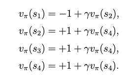
First, we can calculate the state values based on the given policy, like this:

Second, we can calculate the action values for each state. Here we only take state $s_1$ as an example.
Here we have to emphasize the concept of action value again: it is the expected returns obtain at a given state by conducting a certain action.

Obviously, $a_3$ is the greatest action.
For every $s \in \mathcal{S}$ , the elementwise expression of the BOE (a set of linear equation for updating state value) is
$$
v(s) = \max_{\pi(s) \in \Pi(s)} \sum_{a\in \mathcal{A}}\pi(a|s) (\sum_{r\in\mathcal{R}}p(r|s, a)r + \gamma \sum_{s’\in \mathcal{S}}p(s’|s, a)v(s’)) = \max_{\pi(s) \in \Pi(s)}\sum_{a\in\mathcal{A}}\pi(a|s)q(s, a)
$$
$\pi(s)$ is a policy for state $s$, $\Pi(s)$ is the set of all possible policies for $s$
Although the BOE has two unknown variables $v(s)$ and $\pi(a|s)$, they can be solved one by one.
Because of the structure of this Equation, we can be inspired by the below example!
Here we have $\sum_a \pi(a|s) = 1$, we have
$$
\sum_{a\in \mathcal{A}}\pi(s|a)q(s, a) = \sum_{a\in \mathcal{A}}\pi(s|a) \max_{a\in \mathcal{A}} q(s, a) = \max_{a\in \mathcal{A}}q(s, a)
$$
where equality is achieved when
Greedy Optimal Policy
this is an optimal policy for solving the BOE $$ \pi(a|s) = \begin{cases} 1, \quad a = a^*\\0, \quad a \neq a^*\end{cases} $$ The matrix-vector form of BOE is $$ v = \max_{\pi \in \Pi}(r_\pi + \gamma P_\pi v) $$ it can be expressed as $$ f(v) = \max_{\pi \in \Pi}(r_\pi + \gamma P_\pi v) $$ therefore, we only need to achieve $v = f(v)$, here we have to use Contraction Mapping Theorem (Fixed Pointed Theorem). Consider a function $f(x)$, where $x \in \mathbb{R}^d$ and $f: \mathbb{R}^d \rightarrow \mathbb{R}^d$. The point $x^*$ is called fixed point if $f(x^*) = x^*$. Therefore the function $f$ is the contraction mapping, if there exists $\gamma \in(0, 1)$ $$ ||f(x_1)-f(x_2)|| \leq \gamma ||x_1 - x_2|| $$Theorem 3.1 (Contraction Mapping Theorem). For any equation that has the form $x =f(x)$ where $x$ and $f(x)$ are real vectors, if $f$ is a contraction mapping, then the following properties hold.
- Existence: There exists a fixed point $x^*$ satisfying $f(x^*)=x^*$.
- Uniqueness: The fixed point $x^*$ is unique.
- Algorithm: Consider the iterative process: $x_{k+1} = f(x_k)$
solving optimal state values
Therefore, for the BOE $v = f(v) = \max_{\pi \in \Pi}(r_\pi + \gamma P_\pi v^*)$. $v^*$ is the fixed point. There always exists a unique solution $v^*$, which can be solved iteratively by $$ v_{k+1} = f(v_k)= \max_{\pi \in \Pi}(r_\pi + \gamma P_\pi v_k) $$solving optimal policy
after we obtain the optimal state values $v^*$, we can easily obtain $\pi^*$ by solving $$ \pi^* = arg\max_{\pi\in \Pi} (r_\pi + \gamma P_\pi v^*) $$Then
$$ v^* = r_{\pi^*} + \gamma P_{\pi^*}v^* $$Greedy Optimal Policy
For any $s \in \mathcal{S}$, the deterministic greedy policy
$$ \pi(a|s) = \begin{cases} 1, \quad a = a^*\\0, \quad a \neq a^*\end{cases} $$ Here, $a^*(s) = arg \max_a q^*(a, s)$ , where $$ q^*(s, a) = \sum_{r\in \mathcal{R}}p(r|s, a)r + \gamma \sum_{s' \in \mathcal{S}}p(s'|s, a)v^*(s') $$