RL Note 7: Policy Gradient Method

Policy Gradient Method

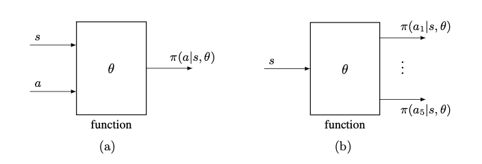
value-based → policy-based. In this case, the policy can be written as $\pi (a|s, \theta)$, where $\theta \in \mathbb{R^m}$ is a parameter vector. This means that we can also use function to represent the policy. Function-represented policies optimal policies can be obtained through policy gradient method, which is policy-based method. It is more efficent for handling larget spaces.

1. select a metric.
2. optimize it through using gradient-ascent algorithm.

​

• Metric 1: Average state value

  $$ \bar{v}_\pi = \sum_{s\in \mathcal{S}}d(s)v_\pi(s) $$

  where $d(s)$ is the weight of state $s$. It satisfies $d(s) \geq 0$ for any $s \in \mathcal{S}$ and $\sum_{s\in \mathcal{S}}d(s)=1$

  If we interpret $d(s)$ as the probability distribution of $s$, The metric will be

  $$ \bar{v}_\pi = \mathbb{E}_{S \sim d}[v_\pi(S)] $$

  We can treat all the states equally important by selecting the $d_0(s) = 1/|\mathcal S|$ or we can only interest in only one state $d_0(s_0) = 1, d_0(s\neq 0) = 0$. If the $d$ is dependent with policy $\pi$ then we could use the stationary distribution.

  $$
  d_\pi^T P_\pi =d_\pi^T
  $$

  The metrics can also be defined like this

  $$ J(\theta) = \lim_{n\rightarrow \infty}\mathbb{E}[\sum_{t=0}^n \gamma^t R_{t+1}] = \mathbb{E}[\sum_{t=0}^{\infty}\gamma^tR_{t+1}] $$ $$ \mathbb{E}[\sum_{t=0}^{\infty}\gamma^tR_{t+1}] = \sum_{s\in \mathcal{S}}{d(s)}\mathbb{E}[\sum_{t=0}^{\infty}\gamma^t R_{t+1}|S_0=s] = \sum_{s\in \mathcal{S}}d(s)v_\pi(s) = \bar{v}_\pi = d^T v_\pi $$ ​

• Metrics 2: Average reward

​ $$ \bar{r}_\pi = \sum_{s\in \mathcal{S}}d_\pi (s)r_\pi(s) = \mathbb{E}_{S\sim d_\pi}[r_\pi(S)] $$ ​

​ here the $d_\pi$ is the stationary distribution
$$
r_\pi(s) = \sum_{a \in \mathcal{A}} \pi(a|s, \theta)r(s, a) = \mathbb{E}_{\mathcal{A}\sim \pi(s, \theta)}[r(s, A)|s]
$$

​ here $r(s, a) = \mathbb{E}[R|s, a] = \sum_r rp(r|s, a)$

$$
J(\theta) = \lim_{n\rightarrow\infty} \frac{1}{n} \mathbb{E} [\sum_{t=0}^{n-1 }R_{t+1}]
$$

$$
J(\theta) = \lim_{n\rightarrow\infty} \frac{1}{n} \mathbb{E} [\sum_{t=0}^{n-1 }R_{t+1}] = \sum_{s\in \mathcal{S}}d_{\pi}(s)r_{\pi}(s) = \bar{r}_\pi
$$

Policy Gradient Theorem

$$
\nabla_{\theta}J(\theta) = \sum_{s\in \mathcal{S}}\eta(s)\sum_{a\in\mathcal{A}}\nabla_\theta \pi(a|s, \theta)q_\pi(s, a)
$$

The compact form in terms of expectation is

$$ \nabla_\theta J(\theta) = \mathbb{E}_{S\sim \eta, A \sim \pi(S, \theta)}[\nabla_\theta \ln \pi (A|S, \theta )q_\pi(S, A)] $$

Derivation of the gradients in the discounted case

$$
v_\pi (s) = \mathbb{E} [R_{t+1} + \gamma R_{t+2} + \cdots | S_t = s]
$$

$$
q_\pi(s, a) = \mathbb{E} [R_{t+1} + \gamma R_{t+2} + \cdots | S_t = s, A_t = a]
$$

It holds that $v_\pi(s) = \sum_{a\in \mathcal{A}}\pi(a|s) q_\pi(s, a)$. We can also shows that $\bar{r}_\pi(\theta)$ and $\bar{v}_\pi(\theta)$ are the same expression. $$ \bar{r}_\pi = (1 - \gamma )\bar{v}_\pi $$ Know that $\bar{v}_\pi(\theta) = d_\pi^Tv_\pi$ and $\bar{r}_\pi (\theta) = d_\pi^Tr_\pi$, and the Bellman equation is $v_\pi =r_\pi + \gamma P_\pi v_\pi$. $$ \bar{v}_\pi = \bar{r}_\pi + \gamma d_\pi^T P_\pi v_\pi = \bar{r}_\pi+ \gamma \bar{v}_\pi $$

​

​

MC Policy Gradient (REINFORCE)

The gradient ascent to maximizing $J(\theta)$ is

$$ \theta_{t+1} = \theta_t + \alpha \nabla_\theta J(\theta_t) =\theta_t + \alpha \mathbb{E}_{S\sim \eta, A \sim \pi(S, \theta)}[\nabla_\theta \ln \pi (A|S, \theta )q_\pi(S, A)] $$

Apply SGD
$$
\theta_{t+1} =\theta_t + \alpha [\nabla_\theta \ln \pi (a_t|s_t, \theta )q_t(s_t, a_t)]
$$

where $q_t(s_t,a_t)$ is the approximation of $q_\pi(s_t,a_t)$ . If it is obtained by MC, the algorithm is called REINFORCE.

$$
\theta_{t+1} =\theta_t + \alpha (\frac{q_t(s_t,a_t)}{\pi(a_t|s_t, \theta_t)})\nabla_\theta \pi(a_t|s_t, \theta)
$$
Algorithm: REINFORCE (Policy Gradient by MC Learning )

Initialization: Initial parameter $\theta$ ; $\gamma \in (0, 1)$ ; $\alpha > 0$

Goal: Learn an optimal policy for maximizing $J(\theta)$

For each episode, do

• Generate an episode ${s_0, a_0, r_1, \cdots, s_{T-1}, a_{T-1}, r_T}$ following $\pi(\theta)$

• For $t = 0, 1, \cdots, T-1$

  • Value update: $q_t(s_t, a_t) = \sum_{k=t+1}^T \gamma^{k-t+1} r_k$
  • Policy update: $\theta \leftarrow \theta + \alpha \nabla_\theta \ln \pi(a_t|s_t, \theta)q_t(s_t, a_t)$